Doing math the cool way (GNU Octave)

I remember in college, there was one math professor that did the problem examples on the whiteboard, but when he got stuck he will real quick go to his laptop, open GNU Octave and type in a short formula that will solve him the whole problem. And then he would say: "Ah i see where i went wrong", then he would go back to the whiteboard and complete the problem. That seemed so cool to me. But at that time i did not try doing anything like it because it seemed hard, and i have more on my plate than math problems. But now when I'm a bit older and smarter, i guess i can try a few things.
octave:14> 5+2
ans = 7
octave:15> 2^2
ans = 4
octave:16> sqrt(9)
ans = 3
octave:17> mod(21, 5)
ans = 1
To clear the command window type "clc", and to clear the variables type "clear all". Let's say the goal is to solve problem of two equations and two unknown variables then we use matrix method Ax = b (dont know how that method is called...).
Let's say we have:
2x+3y=8 and x-y=1
we turn that into matrices:
#Left of the equal sign
A=[2,3;
1,-1];

#Right of the equal sign
b=[8; 1]
And then we solve for x by doing:
x = inv(A) * b
ans =

   2.2000
   1.2000
This is the fastest way to soling this kind of equations, and i believe it's the simplest way for computers to solve it, however i don't like it that much. But it is what it is. Onwards.
It's possible to quickly make arrays with lots of numbers, actually in last post about proportional regulators there was a graph that was made with those.
Example:
t=0:1:20
This will make array that goes from 0 to 20 in increments of 1:
octave:1> t=0:1:20
t =

    0    1    2    3    4    5    6    7    8    9   10   11   12   13   14   15   16   17   18   19   20
And on top of that it's possible to perform operations on that array:
octave:1> t=0:1:20
t =

    0    1    2    3    4    5    6    7    8    9   10   11   12   13   14   15   16   17   18   19   20

octave:2> t+2
ans =

    2    3    4    5    6    7    8    9   10   11   12   13   14   15   16   17   18   19   20   21   22

octave:3> t*3
ans =

    0    3    6    9   12   15   18   21   24   27   30   33   36   39   42   45   48   51   54   57   60

octave:4>
Now i feel stupid for showing this, it feels like a second nature to everyone, so for the end i will show a little of control system functions. There is package called Control and is used specifically for simulating control systems. It's not that i know much about it, in fact i don't, but I'm trying to learn, and it seems so cool to use this tool.
Here is the proportional regulator, aka P regulator:
octave:13> pkg load control
octave:14> t = 0:0.01:10;
octave:15> Kp = 2.0;
octave:16> r = 1.0;
octave:17> sys = tf(Kp, [1, 1+Kp]);
octave:18> y=lsim(sys, r*ones(size(t)), t);
octave:19> plot(t, y, 'b', t, r*ones(size(t)), 'r--');
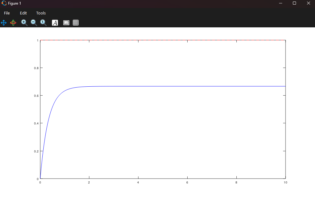
And it made a graph. It's great. I forgot something earlier. The command "who" is to show what variables are currently in use, and then "clear all" is to delete them all.
That's it, thanks for reading.